Tutorial on Calculating a Marmoset Brain Connectivity Matrix Using Brain/MINDS DWI Data and the Brain/MINDS 3D Digital Marmoset Brain Atlas.
By Connectome Analysis Unit. Last Updated 2024/3/29.
Introduction
This tutorial will show you how to calculate a marmoset brain connectivity matrix using DWI data from the Brain/MINDS NA216 dataset and the Brain/MINDS 3D digital brain atlas (BMA 2019). The resulting matrix will estimate the strength of structural connectivity between anatomical brain regions defined in the atlas. This tutorial will use the popular DSI Studio for all of the calculations. The tutorial shows the basic steps for connection matrix construction and is for demonstration purposes only, we make now claims on the quality of the connectivity results.
Software
We will use DSI Studio for carrying out our analysis. Please download the appropriate version from the website and install it. This tutorial was tested on the Chen September 13 2023 version, running on macOS 13.6.4.
Download Data
We will download and use the following data for the individual with ID: 001 from the NA216 dataset:
- The in-vivo diffusion weighting image: dwi_001.nii
- The b-value and b-vector files for the above scan NA216.bval and NA216.bvec. We also renamed these files to match the name of the individual data (dwi_001.bval and dwi_001.bvec) and placed them in the same folder on the computer as the dwi_001.nii file for easy loading into DSI Studio.
- The in-vivo fractional anisotropy image: dtiFA_001.nii.gz
- The BMA 2019 atlas mapped to the dwi_001.nii data: Label_BMA2019_DTI_001.nii.gz
Step 1: Load the DWI source data into DSI Studio
- Open DSI Studio and click the ‘Step T1: Open Source Images’ button. From the file system select and load a DWI dataset, in our case we chose brain ID: 001, dwi_001.nii. DSI Studio recognizes the renamed .bvec and .bval files as a single dataset and will automatically load the b-value and b-vector information together with the dwi_001.nii file.
- Click ‘Sort b-table‘ (to be safe).
- Click ‘OK‘, then a SRC file, a file in the DSI Studio format, is created (dwi_001.nii.src.gz).
Step 2: Reconstruct per-voxel fiber orientations
- Click the ‘Step T2: Reconstruction’ button.
- Choose dwi_001.nii.src.gz as the data to reconstruct.
- A new window will be displayed showing a red segmentation mask that highlights the brain region of interest to be processed.
- We can automatically improve this mask by clicking ‘U-Net Mask’ to remask the data.
- Select ‘Check b-table’ so that DSI Studio does a sanity check on the orientations of the b-table data.
- Choose the GQI reconstruction method.
- Click ‘Run Reconstruction’.
- After completion, close the window and you will see that a file, dwi_001.nii.src.gz.gqi.0.6.fib.gz, has been created. This contains the per-voxel fiber orientations.
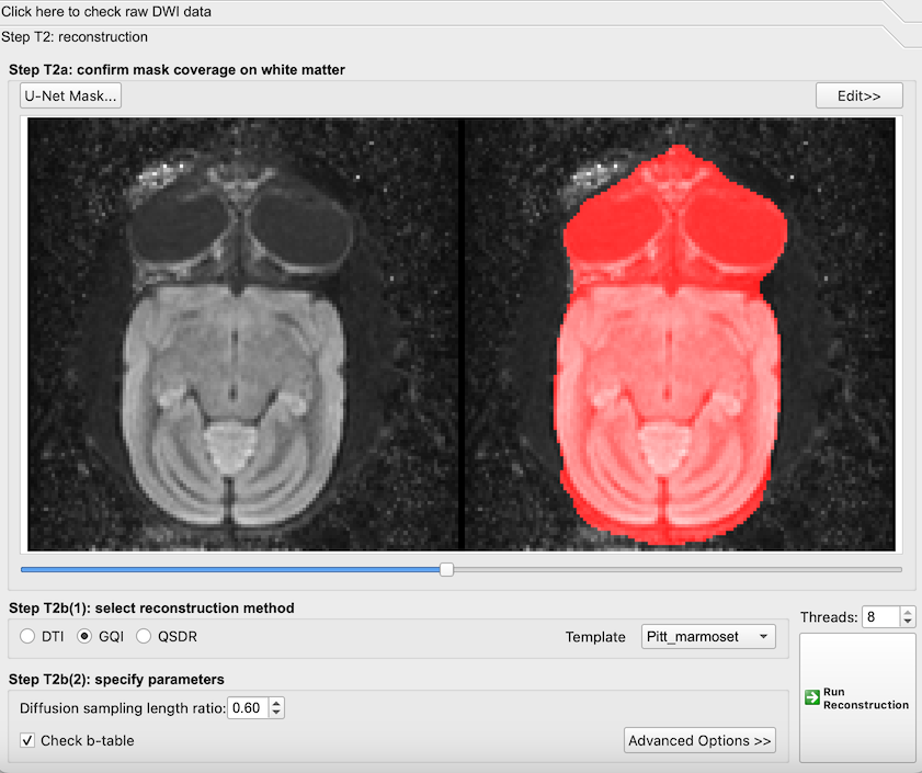
The default masking of the DWI data when loading the data. Axial view of the marmoset brain.
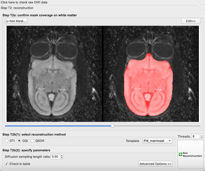
The mask after U-Net refinement. Notice that the mask now follows the boundaries of the brain.
Step 3: Generate whole brain fiber tracks
- Choose ‘Step T3: Fiber Tracking & Visualization’, this will open a new window that will allow you to do fiber tracking, connection matrix calculation, and visualize the results.
- Under the ‘Step T3c: Options’ panel on the right, under ‘Tracking Parameters’ use the default settings but change ‘Seeds’ to ‘Tracts’ under the ‘Terminate if’ condition.
- Click the ‘Fiber Tracking’ button under Step T3d: Tracts’ and wait for the software to generate a set of whole brain fiber tracks (a tractogram).
- Save the resulting track data to file (in this tutorial the file is named whole_brain.tt.gz).
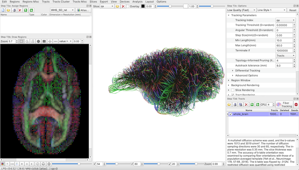
A view of the ‘Step T3: Fiber Tracking & Visualization’ window. The figure shows a 3D visualization of the whole brain fiber tracking result (middle panel) and an axial view of color-coded per-voxel fiber orientations overlaid onto the brain’s DWI b0 contrast.
Step 4: Process the brain atlas to extract anatomical ROIs
In order to generate a connectivity matrix we need to use a reference atlas that can provide us with parcellations (regions of interest, or ROIs) for each anatomical brain region. Luckily we have the Brain/MINDS atlas (BMA 2019) version mapped to this DWI dataset.
DSI Studio requires each brain region ROI to be loaded as a set of files, so in order to use the atlas data, we made a script that will load the atlas data (NIfTI file) and generate one NIfTI file per brain region (we call these regions of interest (ROIs)). The script takes the atlas data and a lookup table mapping IDs to region names to generate ROIs with the region name appended to the filename. These files are output into a folder ‘rois’. The code is shown below:
					import numpy as np
import SimpleITK as sitk
import re

region_list = []
with open("./input/bma-1-clut.ctbl") as f:
    for line in f.readlines():
        elements = line.split()
        abbrev = re.findall(r"\(.*?\)", line)
        if len(abbrev) > 0:
            region_list.append([elements[0], abbrev[len(abbrev) - 1]])

print(region_list)

img = sitk.ReadImage("./input/Label_BMA2019_DTI_001.nii.gz")
nda = sitk.GetArrayFromImage(img)
id_list = np.unique(nda)

print(len(id_list))
for i in range(len(id_list)):
    nda_working = nda.copy()
    nda_working[nda_working != id_list[i]] = 0
    img_out = sitk.GetImageFromArray(nda_working)
    img_out.CopyInformation(img)
    abbrev = "nothing"
    for j in range(len(region_list)):
        if int(region_list[j][0]) == id_list[i]:
            abbrev = region_list[j][1]
            abbrev = abbrev.replace("/", "-")
    if abbrev != "nothing":
        sitk.WriteImage(
            img_out, "./rois/roi-" + str(int(id_list[i])) + "-" + abbrev + ".nii.gz"
        )
Before we load the ROIS, first we need to load the reference volume image to provide a space for the data. We will use the fractional anisotropy volume provided:
- At the top options panel, go to ‘Slices’->’Insert Other Images’ and choose ‘dtiFA_001.nii.gz’. The file should load and you should see the visualization update.
Now load the regions:
- In the panel ‘Step T3a: Assign Regions’, click the folder icon.
- Navigate to the directory with the generated individual ROI files, select them all, then click open.
- At the top options panel, choose ‘Regions’, and click ‘Check All’.
- Under the ‘Step T3c: Options’ panel, deselect ‘Slice Rendering’ to easily visualize the regions and show that they align correctly with the generated tracts.
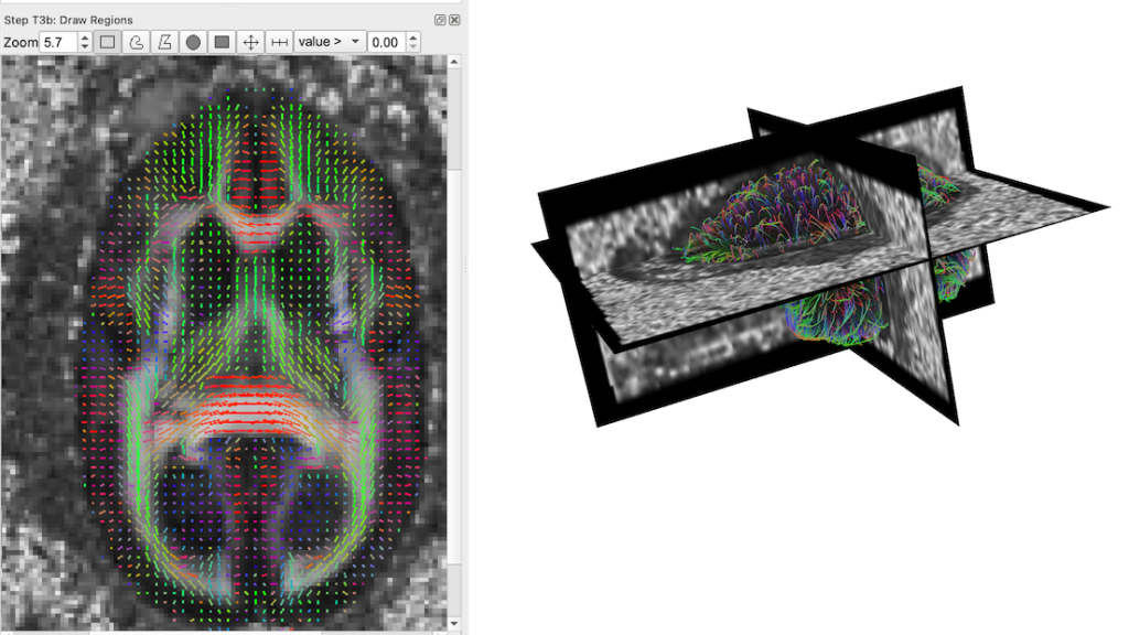
A visualization of the fractional anisotropy volume image. Left: an axial plane with fiber orientations overlaid. Right: a 3D view visualizing orthogonal planes through the FA volume along with the generate fiber tracks.
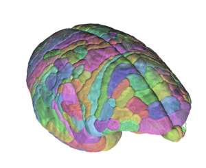
A semi-transparent 3D visualization of the brain atlas anatomical ROIs on top of the whole brain fiber tracking.
Step 5: Generate a connectivity matrix
Under ‘Step T3d: Tracts’, right click the ‘whole_brain’ tractogram and click ‘connectivity matrix’, this will generate a connectivity matrix using the checked ROIs. A text description of the settings used for the matrix is generated, for this tutorial this was as follows:
A multishell diffusion scheme was used, and the b-values were 1013 and 3019 s/mm². The number of diffusion sampling directions were 30 and 60, respectively. The in-plane resolution was 0.35 mm. The slice thickness was 0.7 mm. The accuracy of b-table orientation was examined by comparing fiber orientations with those of a population-averaged template (Yeh et al., Neuroimage 178, 57-68, 2018). The b-table was flipped by .012fz. The restricted diffusion was quantified using restricted diffusion imaging (Yeh et al., MRM, 77:603–612 (2017)). The diffusion data were reconstructed using generalized q-sampling imaging (Yeh et al., IEEE TMI, ;29(9):1626-35, 2010) with a diffusion sampling length ratio of 0.6. A deterministic fiber tracking algorithm (Yeh et al., PLoS ONE 8(11): e80713, 2013) was used with augmented tracking strategies (Yeh, Neuroimage, 2020 Dec;223:117329) to improve reproducibility. The anisotropy threshold was randomly selected. The angular threshold was randomly selected from 15 degrees to 90 degrees. The step size was set to voxel spacing. The fiber trajectories were smoothed by averaging the propagation direction with a percentage of the previous direction. The percentage was randomly selected from 0% to 95%. Tracks with length shorter than 10 or longer than 60 mm were discarded. A total of 1000000 tracts were calculated. parameter_id=c9A99193Fb803Fcb803Fb2041b704240420Fca01ba02baCDCC4C3Ec Shape analysis (Yeh, Neuroimage, 2020 Dec;223:117329) was conducted to derive shape metrics for tractography.
ROIs was used as the brain parcellation, and the connectivity matrix was calculated by using count of the connecting tracks. The connectivity matrix and graph theoretical analysis was conducted using DSI Studio (http://dsi-studio.labsolver.org).
The connectivity matrix and calculated network measures can be saved from the modal window that appears. From here the connection matrix can also be regenerated using different parameter settings. The list of network measures that gets generated is described here. We can then go ahead and load and analyze the connectivity matrix in software of our choosing. As an example, the following figure displays the log_10 of the connectivity matrix visualized in python using matplotlib:
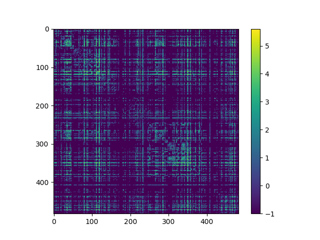
The code to generate the figure was as follows:
					import numpy as np
import matplotlib.pyplot as plt
import scipy.io as sio

mat_contents=sio.loadmat('whole_brain_ROIs.mat')
connectivity=mat_contents['connectivity']

plt.imshow(np.log10(connectivity+0.1))
plt.colorbar()
plt.show()
Now that you have had a taste of marmoset brain connectivity matrix estimation, we encourage you to explore the DSI Studio website for further information on how to carry out a more involved study using the software and the Brain/MINDS data.
The data, scripts and generated files used for this tutorial are available for download here.