Technical Details
1) Injection map
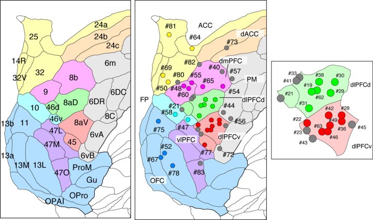
We subdivided the frontal areas into nine subdivisions, namely, ACC (anterior cingulate cortex), dACC (dorsal ACC), dmPFC (dorsomedial PFC), dlPFCd (dosolateral PFC-dorsal), dlPFCv(dorsolateral PFC-ventral), FP (frontal pole), vlPFC (ventrolateral PFC), OFC (orbitofrontal cortex) and PM (premotor cortex). The left panel indicates which cortical areas correspond to these nine subdivisions. The positions of 44 injections are shown on the center and the right panels with injection number.
2) AAV tracer

We used a Tet-Off-based AAV vector system for enhanced expression of the fluorescent proteins for axon labeling. In this system, tTA2 (Tet-Off transactivator) protein is produced in a neuron-specific manner under the control of thy1S promoter. The tTA2 proten binds to the TRE response element and produces a large amount of fluorescent protein, clover, a GFP derivative.
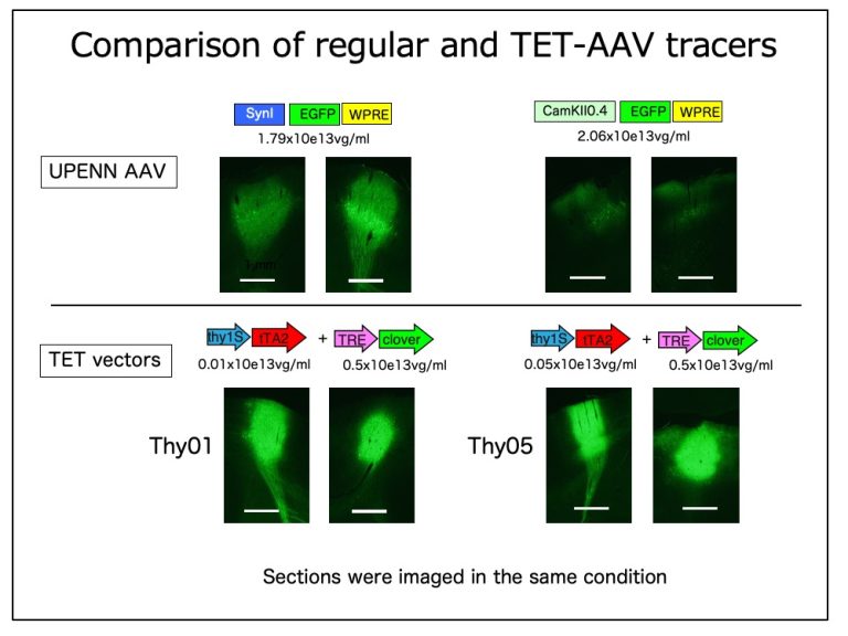
There are several advantages of the TET-tracer compared with the regular AAV GFP tracer. (1) Because of highly enhanced expression, you can get stronger fluorescence with less amount of AAV. After further experiments, we decided that 1x10e12 vg/ml each of TET and TRE vectors leads to saturated expression and used that condition throughout our experiments. (2) Because you can reduce the absolute amount of AAV particles, you can reduce the danger of retrograde labeling. (3) The transduction efficiency of cortical neurons appear to depend on the size of the cells. The regular AAV shows strong expression in the large pyramidal cells in layer 5, but not so much for layer 2/3 pyramidal neurons, leading to less efficient labeling of the corticocortical projections (manuscript in preparation). This tendency was particularly evident in primates. In contrast, TET vectors lead to rather even labeling across layers, which we found suitable for our mapping project. (4) The strong expression requires co-transduction of the same neurons by the two AAV vectors . The spread of the fluorescence is therefore more restricted compared with the regular AAV.
3) Connection matrix
The connection matrices provided on this website show you summaries of the projection intensities in various anatomical regions that originated from 44 injections. We provide these matrices as an aid to (1) find regions that receive projections from the injection of interest and (2) find injections that send projections to the region of interest. The connection matrix is an important primary resource to perform graph analyses, but our data is not currently intended for that purpose for a variety of reasons. When we acquired a more extensive dataset in the ongoing project, we will provide the connection matrix for graph analyses.
Below, we would like to discuss several factors that may confound the interpretation of the connection matrix.
Confounding factors
[ROI/Region of Interest]
The connection matrix is constructed by measuring the intensities of tracer signals in various Region of Interests or ROIs. There are, however, two kinds of complications concerning ROI. First of all, the anatomical boundaries are not necessarily established. Although there exists a global consensus on definitions of major anatomical structures, the anatomical boundaries are often subtle and difficult to determine objectively. Depending on the regions, the “same” areas are designated differently across literature or across species. Conversely, the same names may be used for different structures. Due to developmental history, there exist overall hierarchical relationships among anatomical structures, which lays the basis for anatomical nomenclatures. Nevertheless, such relationships are often compromised because of cell migrations during development. The anatomical annotations are often updated as we gain more information on the structures of interest. Thus, we should regard the ROIs as tentative. Technically, the whole brain analyses as we did in this project use a standard template with defined ROIs. Currently, we use a standard template named “STPT template”, which is a 50µm-isocubic 3D tissue image of Serial Two-photon tomography (STPT) imaging (Skibbe et al. 2022, Watakabe et al. 2021) with three kinds of annotations for the definition of ROIs for measurement. One is the STPT annotation, which is based on the contrast of STPT template (STPT annotation) (Skibbe et al. 2022, Watakabe et al. 2021). The second is the annotation that was transferred from the Brain/MINDS atlas by registration. The third is the annotation that was transferred from the Marmoset Brain Mapping atlas (MBM atlas: https://marmosetbrainmapping.org/) by registration. These are slightly different and we plan to provide different connection matrices for each annotation.
Skibbe et al. 2022: “The Brain/MINDS Marmoset Connectivity Atlas: exploring bidirectional tracing and tractography in the same stereotaxic space” https://www.biorxiv.org/content/10.1101/2022.06.06.494999v1
Watakabe et al. 20211: “Connectional architecture of the prefrontal cortex in the marmoset brain” https://www.biorxiv.org/content/10.1101/2021.12.26.474213v1
The second complication that we need to consider is the technical variabilities associated with registration. Comparison of different samples entirely relies on accurate registration of the sample data to the standard template. This process is susceptible to misregistration, especially when strong fluorescent signals are present near the ROI borders, for example, in the white matter, or in the internal capsule. It is, therefore, necessary to refer to the original image data, when some anomalies are found.
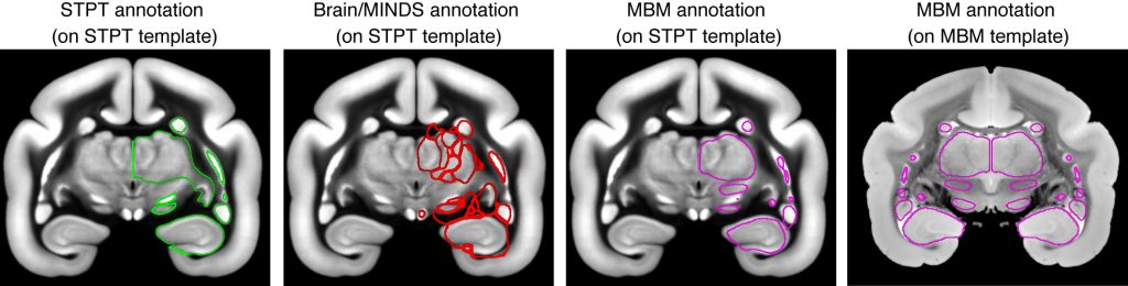
Example images showing differential annotations for the same coronal slice. The thalamus is annotated as a whole in STPT annotation, while it is divided into many subnuclei in Brain/MINDS annotation. LGN is differentially annotated from the “thalamus” in MBM annotation but is included in STPT annotation. These images are good examples showing (1) the same name is used to annotate different structures, (2) Which structures to annotate differ across annotation systems, (3) Misregistration occurs when the annotations are transferred to different templates.
[Injection]
Injections are often difficult to control. We need to consider three types of problems that may affect the connection matrix. One is the leak of the AAV tracer to irrelevant locations, especially when the injections targeted the deep part of the brain. For example, we observed a considerable leak of the tracers in the dorsal brain surface, when we targeted the orbitofrontal cortex (e.g., TT52). In another example, we successfully injected the AAV tracer into A24a without a leak to A24b, but the tracer leaked to the striatum (TT64). The second problem is the imbalance of lamina transduction. Since the projection neurons in different layers exhibit different target specificities, the imbalance at the injection can cause distortions in the target preferences.

The third problem is the difference in the tangential spread. The number of neurons that are directly infected by the AAV tracer can affect the patterns of projections (see below for standardization).

[Intensity measurement and standardization]
The tracer signals are distinguished from the tissue background by machine learning based on the shape and color information. Each positive pixel has a fluorescent value. The intensity of the tracer signals of a unit isocube (50µm x 50µm x 50µm) in the reference space is defined by the number of positive pixels within the isocube multiplied by the fluorescent values. To compare the patterns across different samples, the tracer intensities need to be standardized. Currently, we adopted the standardization based on the maximum intensity value. To be more precise, we excluded the injection sites and their vicinities from standardization, because the AAV-transduced cell bodies emit a saturating amount of fluorescence. This standardization method is effective for evaluating the focal-type projections (Watakabe et al. 2021). On the other hand, it does not adjust the difference in the injection size (see above). For example, the intensity of TT28 is weaker than other samples. An alternative method of standardization would be to standardize by the sum of tracer signals for the cortex or for the entire brain as is performed for the retrograde tracer (e.g., FLN in Markov et al. 2011). We plan to provide such values in the future update.
Watakabe et al. “Connectional architecture of the prefrontal cortex in the marmoset brain. bioRxiv 2021.12.26.474213; doi: https://doi.org/10.1101/2021.12.26.474213
Markov et al. “Weight Consistency Specifies Regularities of Macaque Cortical Networks” Cerebral Cortex (2011) 21:1254
[On the method of intensity measurement]
The connection matrices for the cortical projections show the sum of tracer signals in each ROI, whereas those for the subcortical projections show the averaged intensity. When the ROI is large (e.g., V1), the sum of signals tends to become larger even if the projections are weak and sparse. Conversely, the averaged intensity may show a disproportionately large value for a focal projection to a narrow ROI. It is also possible to show the maximum values for each ROI. In this case, the presence of focal projections is highlighted. It is important to note that there is no “correct” method. The connection matrix provides only one aspect of connectivity, which is a summary of more complex data.